Note

This page was generated from a Jupyter notebook. The original can be downloaded from here.

Duplicates: Find Near Duplicate Data Samples#

Discover near duplicate data samples, which might indicate that there is not enough variation in the dataset.

Please see the doc page on near duplicate discovery and removal for a description of the problem, the Duplicates introspector, and what actions can be taken to improve the dataset.

For a more detailed guide on using all of these DNIKit components, try the Familiarity for Rare Data Discovery Notebook.

1. Setup#

Here, the required imports are grouped together, and then the desired paths are set.

[1]:

import logging
logging.basicConfig(level=logging.INFO)

from dnikit.base import pipeline, ImageFormat
from dnikit.processors import Cacher, ImageResizer, Pooler
from dnikit_tensorflow import TFDatasetExamples, TFModelExamples

# For future protection, any deprecated DNIKit features will be treated as errors
from dnikit.exceptions import enable_deprecation_warnings
enable_deprecation_warnings()

Optional: Download MobileNet and CIFAR-10#

This example uses MobileNet (trained on ImageNet) and CIFAR-10, but feel free to use any other model and dataset. This notebook also uses TFModelExamples and TFDatasetExamples to load in MobileNet and CIFAR-10. Please see the docs for information about how to load a model or dataset. This doc page also describes how responses can be collected outside of DNIKit, and passed into Familiarity via a Producer.

No processing is done at this point! Batches are only pulled from the Producer and through the pipeline when the Dataset Report “introspects”.

[2]:

# Load CIFAR10 dataset
# :: Note: max_samples makes it only go up to that many data samples. Remove to run on entire dataset.
cifar10 = TFDatasetExamples.CIFAR10(attach_metadata=True)

# Create a subset of the CIFAR dataset that produces only automobiles
cifar10_cars = cifar10.subset(datasets=['train'], labels=['automobile'], max_samples=1000)

# Load the MobileNet model
# :: Note: If loading a model from tensorflow,
# :: see dnikit_tensorflow's load_tf_model_from_path method.
mobilenet = TFModelExamples.MobileNet()
mobilenet_preprocessor = mobilenet.preprocessing
assert mobilenet_preprocessor is not None

requested_response = 'conv_pw_13'

# Create a pipeline, feeding CIFAR data into MobileNet,
# and observing responses from layer conv_pw_13
producer = pipeline(
    # Pull from the CIFAR dataset subset that was created earlier,
    # so that only 1000 samples are analyzed in the "automobile" class here
    cifar10_cars,

    # Preprocess the image batches in the manner expected by MobileNet
    mobilenet_preprocessor,

    # Resize images to fit the input of MobileNet, (224, 224) using an ImageResizer
    ImageResizer(pixel_format=ImageFormat.HWC, size=(224, 224)),

    # Run inference with MobileNet and extract intermediate embeddings
    # (this time, just `conv_pw_13`, but other layers can be added)
    # :: Note: This auto-detects the input layer and connects up 'images' to it:
    mobilenet.model(requested_responses=[requested_response]),

    # Max pool the responses before DNIKit processing using a DNIKit Pooler
    Pooler(dim=(1, 2), method=Pooler.Method.MAX),

    # Cache responses
    Cacher()
)

2023-08-03 12:40:58.899809: I metal_plugin/src/device/metal_device.cc:1154] Metal device set to: Apple M1 Pro
2023-08-03 12:40:58.899833: I metal_plugin/src/device/metal_device.cc:296] systemMemory: 32.00 GB
2023-08-03 12:40:58.899836: I metal_plugin/src/device/metal_device.cc:313] maxCacheSize: 10.67 GB
2023-08-03 12:40:58.899863: I tensorflow/core/common_runtime/pluggable_device/pluggable_device_factory.cc:303] Could not identify NUMA node of platform GPU ID 0, defaulting to 0. Your kernel may not have been built with NUMA support.
2023-08-03 12:40:58.899876: I tensorflow/core/common_runtime/pluggable_device/pluggable_device_factory.cc:269] Created TensorFlow device (/job:localhost/replica:0/task:0/device:GPU:0 with 0 MB memory) -> physical PluggableDevice (device: 0, name: METAL, pci bus id: <undefined>)
/private/tmp/dnikit-2.0.0/lib/python3.9/site-packages/keras/src/engine/training.py:3000: UserWarning: You are saving your model as an HDF5 file via `model.save()`. This file format is considered legacy. We recommend using instead the native Keras format, e.g. `model.save('my_model.keras')`.
  saving_api.save_model(
WARNING:tensorflow:Compiled the loaded model, but the compiled metrics have yet to be built. `model.compile_metrics` will be empty until you train or evaluate the model.
INFO:dnikit_tensorflow.TF2:Instantiating TF2 Model
INFO:dnikit_tensorflow.TF2:GPUs Available: 1

(Optional) Perform Dimension Reduction#

Although the Duplicates algorithm can run data with any number of dimensions, there will be improved performance and near identical results if the number of dimensions is reduced. The DNIKit DimensionReduction introspector can be used for this.

[3]:

from dnikit.introspectors import DimensionReduction

dimension_reduction = DimensionReduction.introspect(
    producer, strategies=DimensionReduction.Strategy.PCA(40))
reduced_producer = pipeline(
    producer,
    dimension_reduction,
)

2. Look for duplication in embedding space using Duplicates introspector#

In this step, use the Duplicates introspector to build the clusters of duplicates. This can consume a producer or reduced_producer with no other arguments and give good results.

In some cases, it might be necessary to refine the results. The first way to do this is by modifying the threshold parameter to the introspect() function, of type Duplicates.ThresholdStrategy. For using the percentile or close_sensitivity parameters to the introspect() call. By default the introspector will use a dynamic method to find the bend in the sorted distances. The sensitivity can be controlled with close_sensitivity – the default value is 5. Setting it to 2 will give more duplicates and a sensitivity of 20 will produce fewer. The percentile will use the given percentile in the distance as the “close” threshold. For example a percentile value of 99.5 would take the 99.5th percentile distance and consider that “close” when building thresholds. A lower value would produce more duplicates.

The other way to refine the results is to sort or filter the clusters. They can be sorted by the mean distance to the centroid of the cluster to see the tightest clusters first. For example, filter out clusters larger than N to avoid seeing any very large clusters.

[4]:

from dnikit.introspectors import Duplicates

duplicates = Duplicates.introspect(reduced_producer)

print(f"Found {len(duplicates.results[requested_response])} unique clusters of duplicates.")

INFO:dnikit.base._cached_producer.Cacher:Using cached batches. Attempting to retrieve values..

Found 48 unique clusters of duplicates.

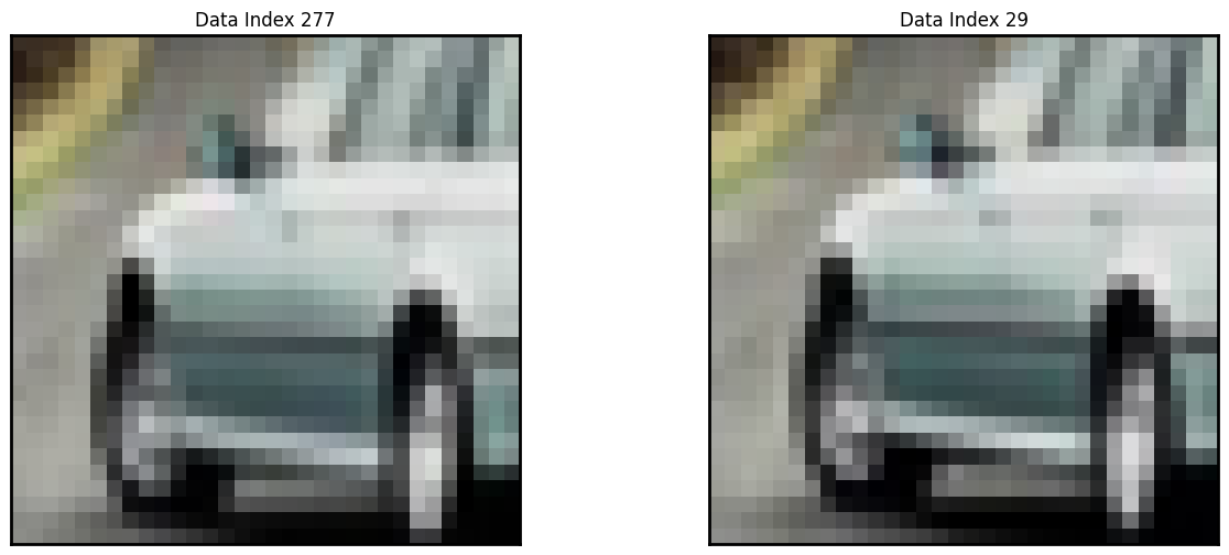
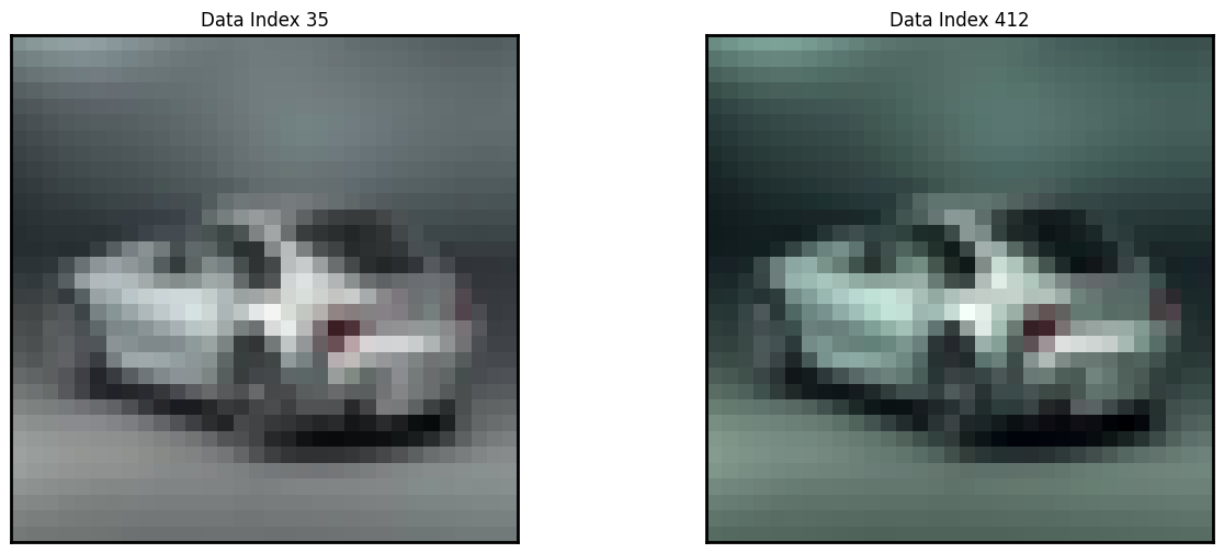
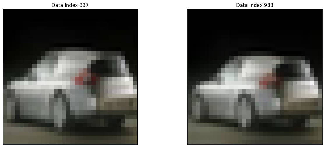
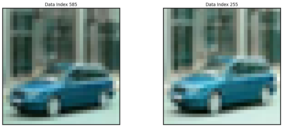
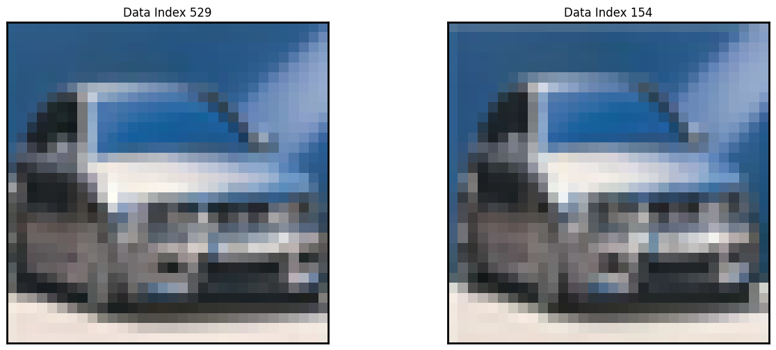
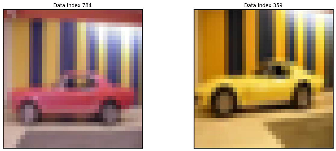
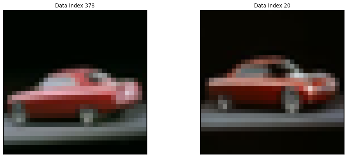
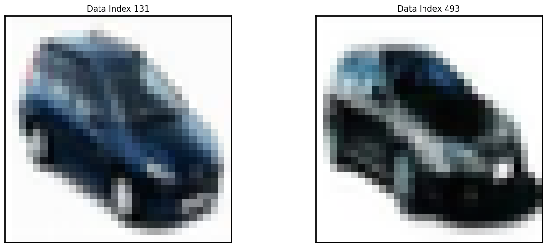
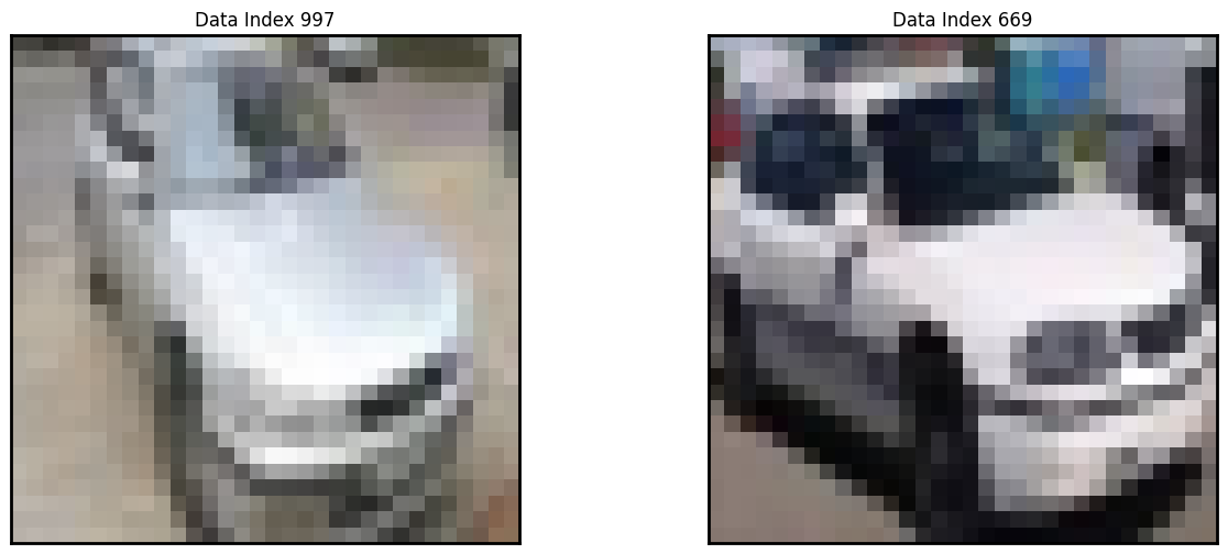
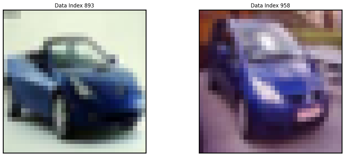
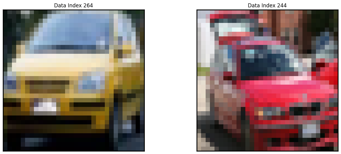
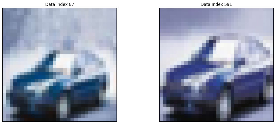
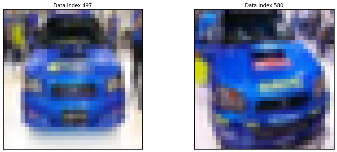
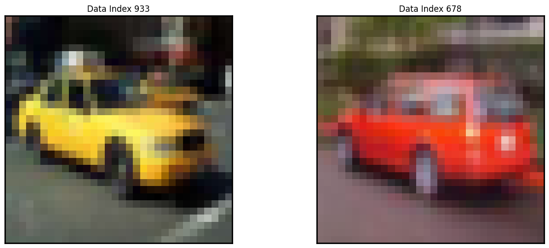
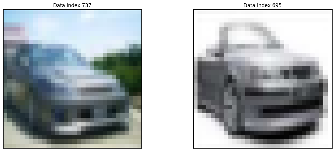
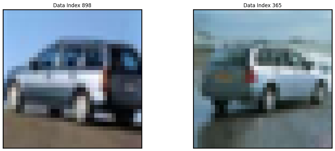
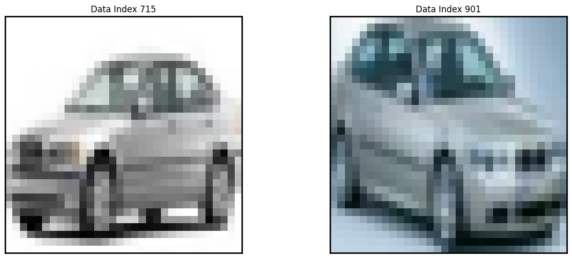
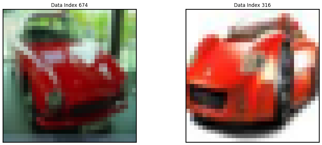
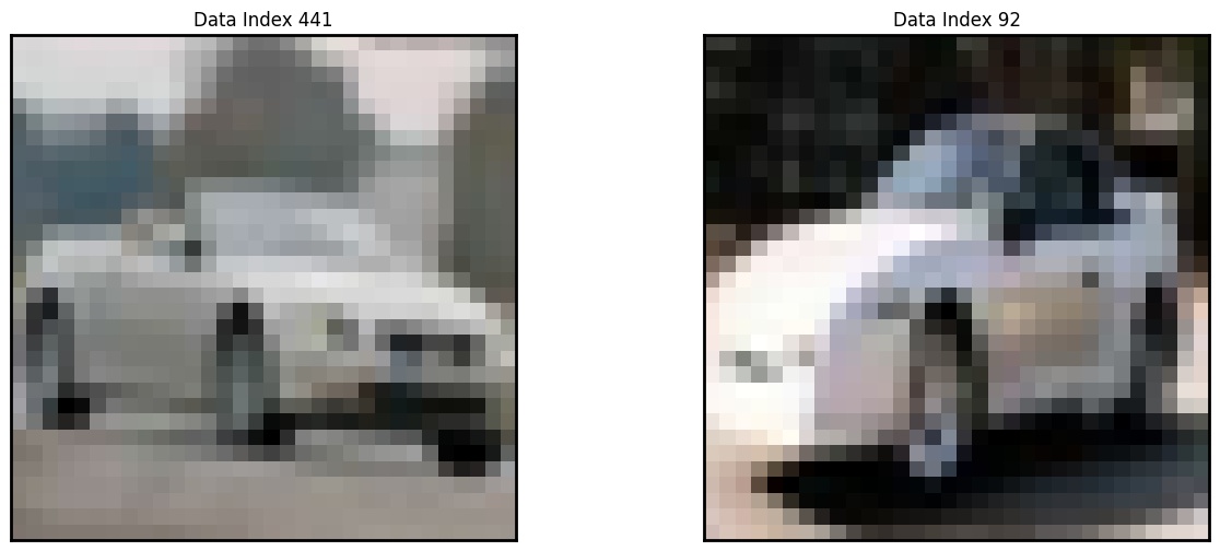
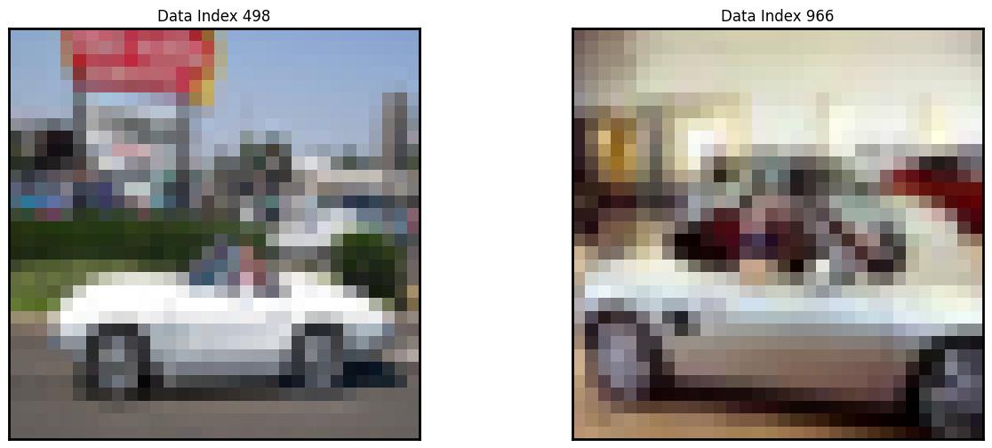
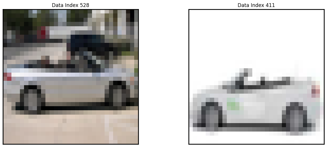
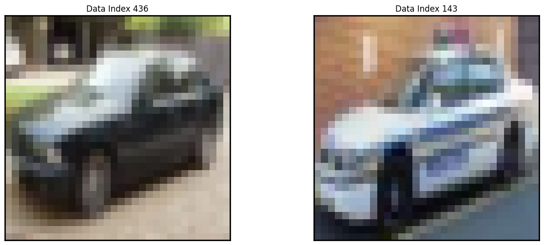
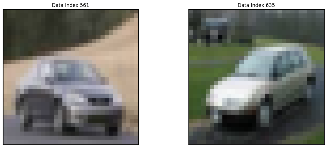
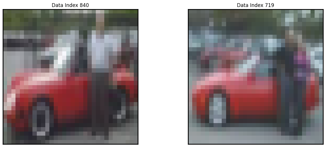
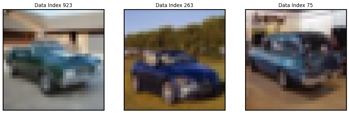
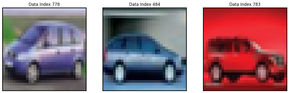
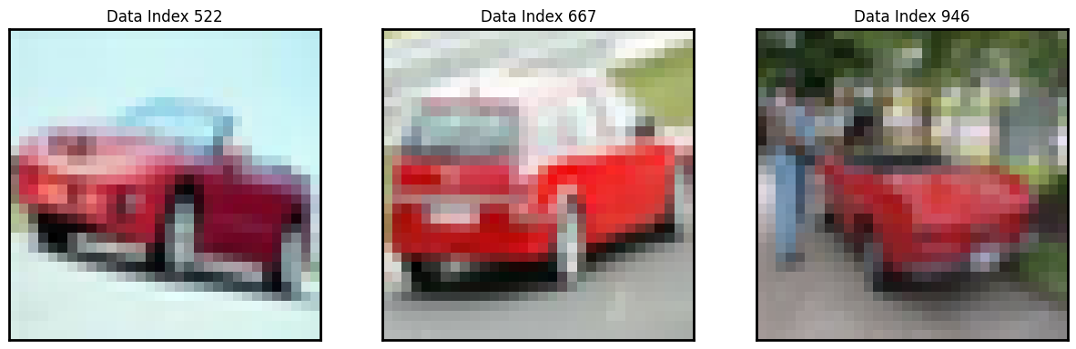
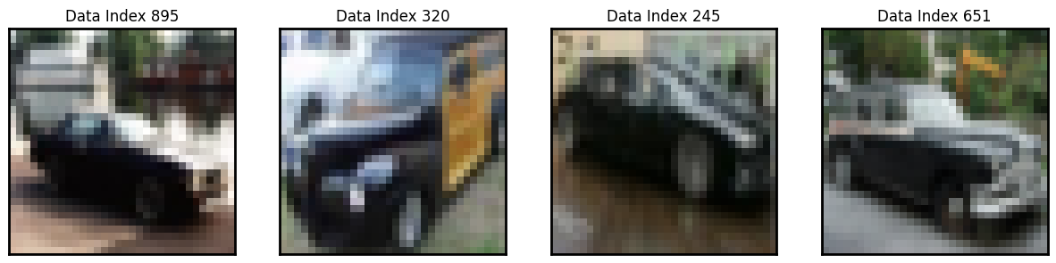
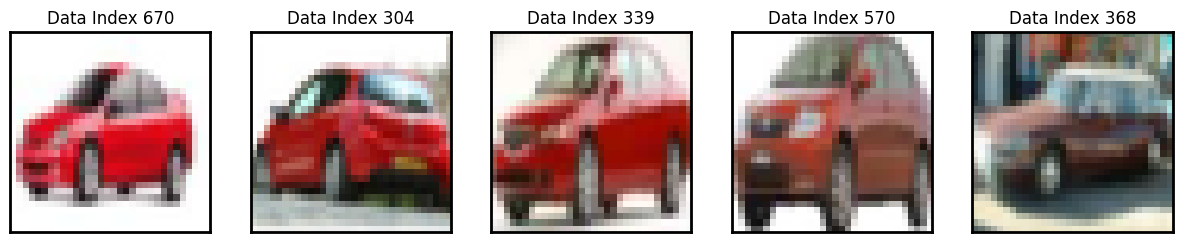
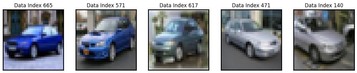
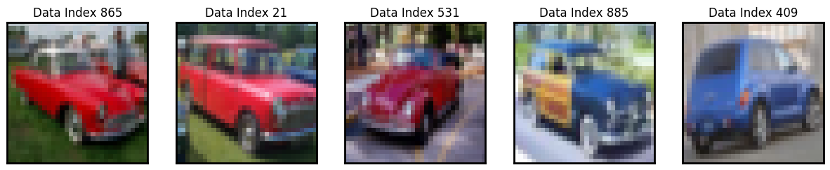
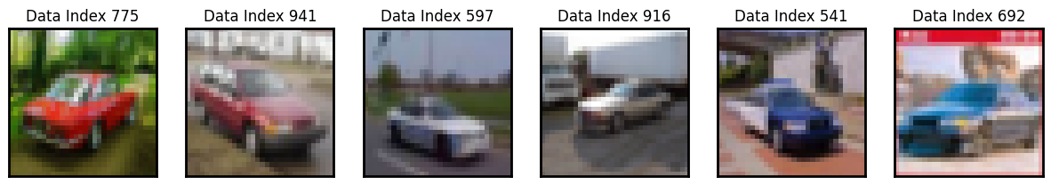
3. Manual analysis of near duplicates - Images#

Now that sets of the most similar images have been computed, visually inspect them and note which data to consider removing before training. All data displayed are unique.

As mentioned in the introduction, it’s not always bad to have similar samples in the dataset. It is bad practice to have duplicates across training and testing datasets, and it’s important to consider the effective training/testing dataset size (including class breakdowns) really is. Remember that slight variation of a data sample for training can be achieved with data augmentation and applied uniformly across all training samples instead of just to a few specific samples as part of the stored dataset.

In general, it’s possible to evaluate the following criteria with the sets of near duplicates:

Set contains train + test images: Are there near identical data samples that span the train and test sets for that class?
Set contains only train images: For near duplicates in the training set, is the network learning anything more by including all near-duplicates? Could some be replaced with good data augmentation methods?
Set contains only test images: For near duplicates in the test set, is there anything new learned about the model if it is able to classify both all the near-duplicate data samples? Does this skew the reported accuracy?

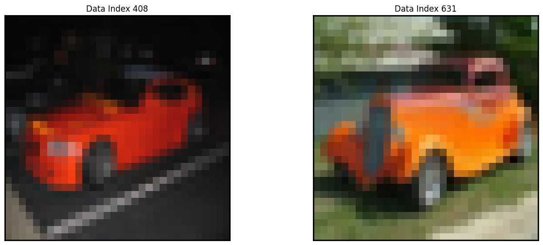
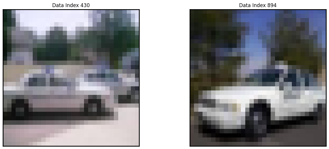
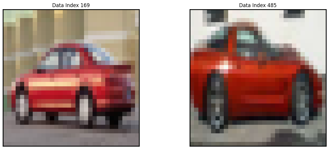
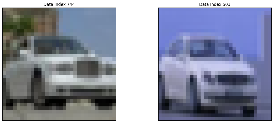
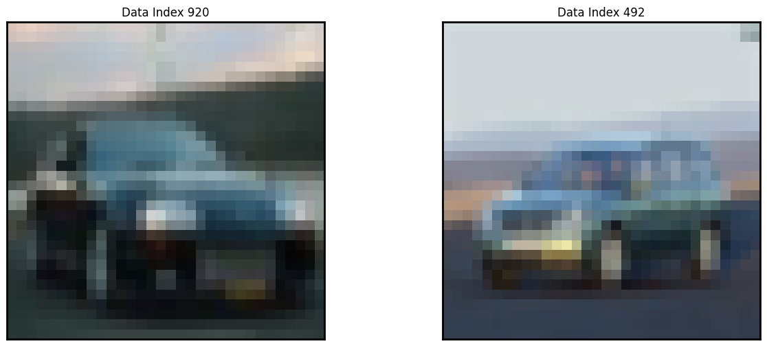
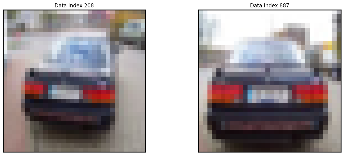
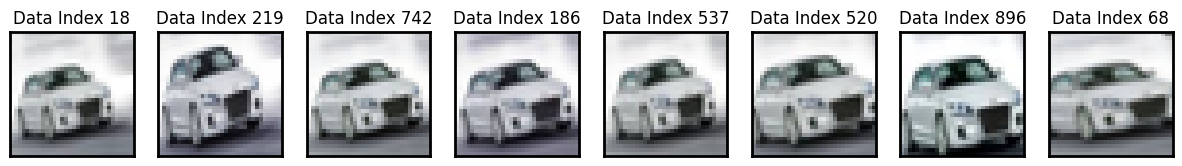
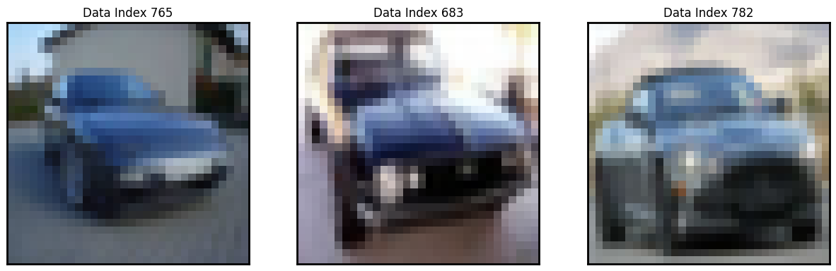
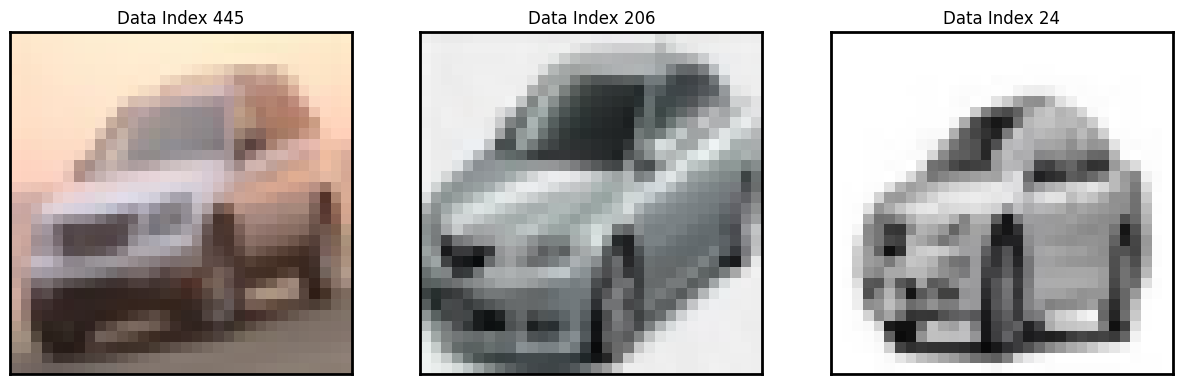
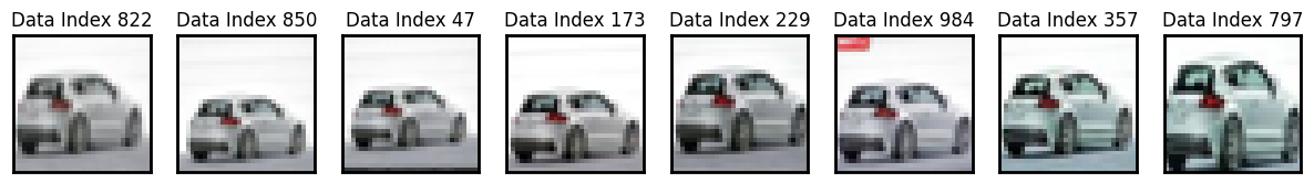
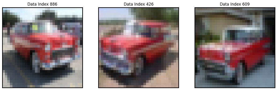
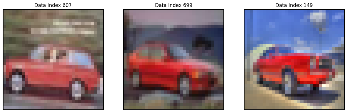
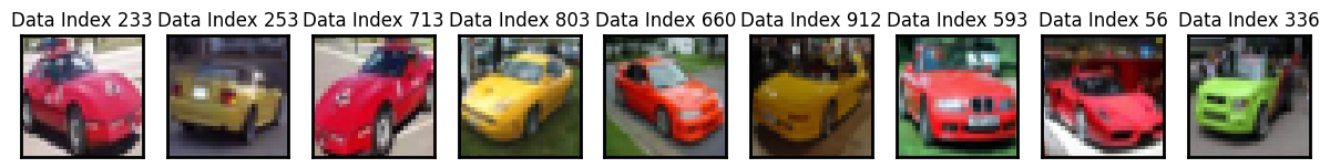
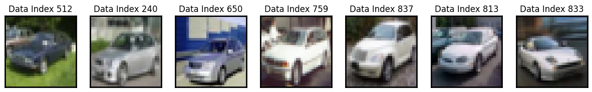
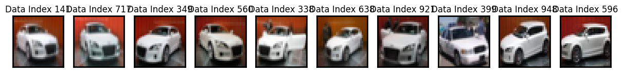
Notice that in the following results, some of the images in the same set look very different (e.g. Cluster 8), but in other lines (e.g. Cluster 1, 2, 3, etc.), the images look nearly identical. This is why it’s important to perform some manual inspection of the data before removing samples.

Even if these images do not appear similar to the human eye, they are closest in the current embedding space, for the chosen layer response name. This can still provide useful information about what the network is using to distinguish between data samples, and it’s recommended to look for what unites the images, and if desired, collect more data to help the network distinguish between the uniting feature.

Anecdote: In this notebook, a small dataset was chosen for efficiency purposes. However, duplicate analysis has been run on all of CIFAR-10, across train and test datasets, and an extremely large number of duplicates has been found. CIFAR-10 is a widely used dataset for training and evaluation purposes, but the fact that there are so many duplicates calls into question the validity of the accuracy scores reported on this dataset for different models, especially with respect to model generalization. Though this is not the first time someone has noticed this issue in the dataset, still, this dataset is widely used in the ML community. It’s a lesson for all of us to always look at the data.

For now, grab all the images into a data structure in order to index into them and grab the data to visualize.

[5]:

images = [
    element.fields['samples']
    for b in cifar10_cars(batch_size=64)
    for element in b.elements
]

[6]:

from dnikit.base import Batch
import matplotlib.pyplot as plt

clusters = duplicates.results[requested_response]
sorted_clusters = sorted(clusters, key=lambda x: x.mean)

for cluster_number, cluster in enumerate(sorted_clusters):
    print(f'Cluster {cluster_number + 1}, mean={cluster.mean}')

    img_idx_list = cluster.batch.metadata[Batch.StdKeys.IDENTIFIER]

    f, axarr = plt.subplots(1, len(img_idx_list), squeeze=False, figsize=(15,6))
    for i, img_idx in enumerate(img_idx_list):
        assert isinstance(img_idx, int), "For this example plot, the identifier should be an int"
        axarr[0, i].imshow(images[img_idx])
        plt.setp(axarr[0, i].spines.values(), lw=2)
        axarr[0, i].yaxis.set_major_locator(plt.NullLocator())
        axarr[0, i].xaxis.set_major_locator(plt.NullLocator())
        axarr[0, i].set_title(f'Data Index {img_idx}')
    plt.show()